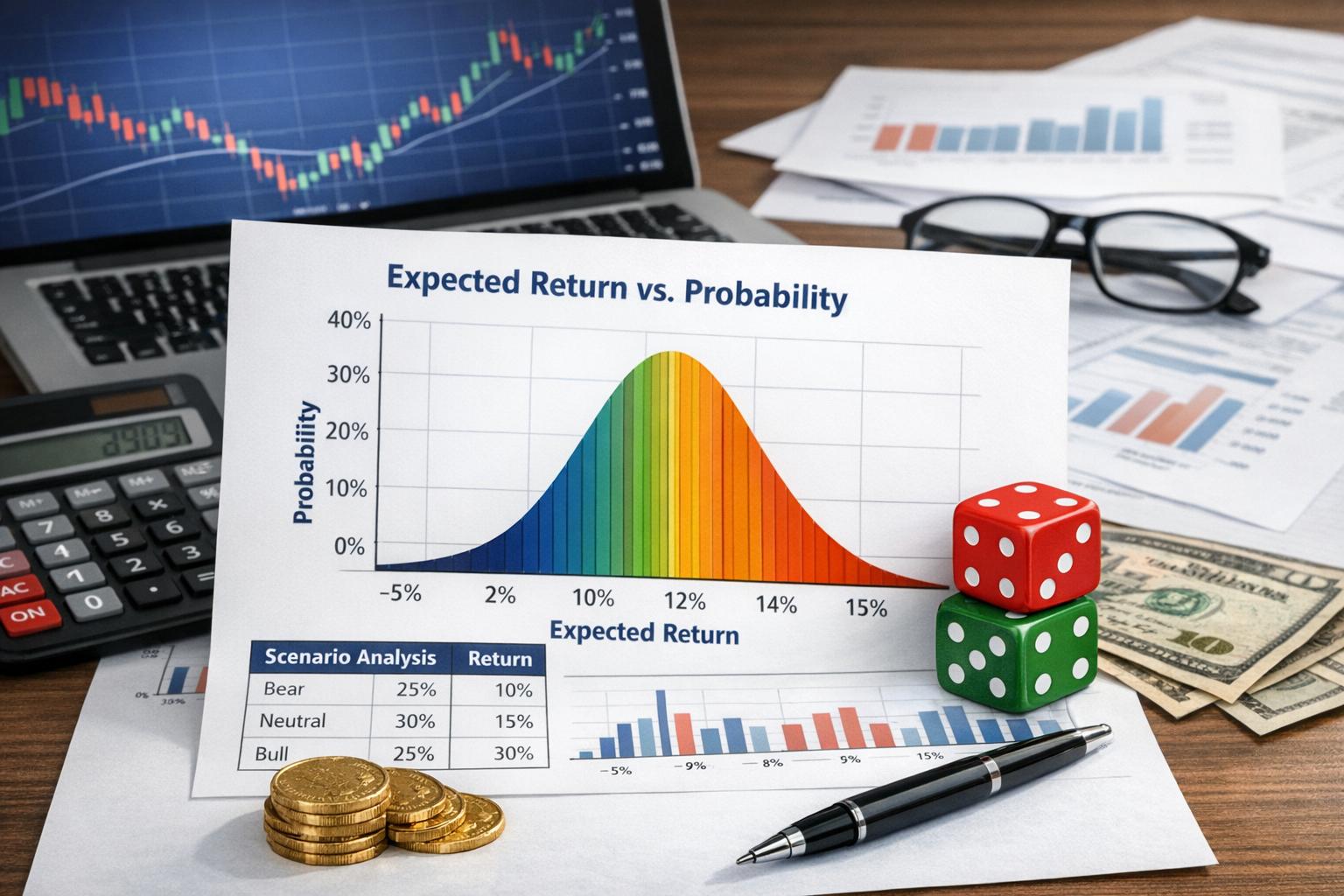
Expected return and probability in finance provide a structured method for assessing uncertain outcomes. Investors cannot know an asset’s future return with certainty, but they can estimate possible results, assign probabilities to them, and calculate an average expected result. That estimate helps compare investments, set portfolio weights, evaluate trades, and decide whether the potential reward justifies the risk.
The calculation itself is straightforward. The harder part is choosing sensible return scenarios and defensible probability estimates. A neat spreadsheet can still produce poor guidance if its assumptions bear little relation to market conditions. Expected return should therefore be treated as an estimate based on available evidence, not as a promised result.
What Is Expected Return?
Expected return is the probability-weighted average of all considered investment outcomes. Each possible return receives a weight based on the estimated chance that it will occur. The resulting figure represents the average return an investor might expect across many repetitions of the same decision.
The general formula is:
E(R) = Σ [P(i) × R(i)]
In this expression:
E(R)is the expected return.P(i)is the probability of outcomei.R(i)is the return associated with outcomei.Σmeans that every probability-weighted outcome is added together.
Probabilities must add up to 100%, or 1.00 when written as decimals. If they do not, the model is incomplete or the inputs need to be normalized.
Suppose a stock has three possible one-year outcomes:
| Scenario | Probability | Return | Weighted Return |
|---|---|---|---|
| Strong trading year | 25% | 30% | 7.5% |
| Ordinary trading year | 50% | 8% | 4.0% |
| Weak trading year | 25% | -18% | -4.5% |
The expected return is:
(0.25 × 30%) + (0.50 × 8%) + (0.25 × -18%) = 7%
A 7% expected return does not mean the stock will earn exactly 7%. In the table above, 7% is not even one of the possible scenario returns. It is the probability-weighted average across the full set of assumptions.
How Probability Works in Financial Analysis
Probability measures the chance that an event will occur. It ranges from 0 to 1, or from 0% to 100%. A probability of zero means the event is treated as impossible within the model. A probability of one means it is treated as certain.
Financial probabilities may come from historical data, option prices, analyst assumptions, economic forecasts, statistical models, or an investor’s own judgment. Each source has weaknesses. Historical frequencies may fail after market conditions change, while personal estimates can reflect optimism, fear, or recent experience.
Objective and Subjective Probability
Objective probability is estimated from observed data. An analyst might review how often a broad equity index produced a negative annual return across several decades. The observed frequency can serve as an initial probability estimate.
Subjective probability comes from judgment. A portfolio manager may estimate the chance of a central bank rate cut after reviewing inflation, employment, and policy statements. Two competent analysts may reach different estimates because they assign different weights to the evidence.
Most real financial models combine both forms. Historical data provides a reference point, while judgment accounts for conditions that the historical sample may not represent well.
Unconditional and Conditional Probability
An unconditional probability estimates the chance of an event without reference to another event. A statement such as “the stock has a 40% chance of gaining more than 10% next year” is unconditional if no other condition is attached.
A conditional probability estimates the chance of an event given that another event has occurred. It is commonly written as:
P(A | B)
This notation means the probability of event A given event B. A financial example could be the probability that bank shares fall given that loan defaults rise above a chosen threshold.
Conditional probability is often more useful than a broad historical average. Asset returns depend on interest rates, economic growth, valuation, liquidity, company earnings, and investor positioning. A probability estimate that accounts for those conditions may be more informative than one based on all periods lumped together.
Expected Return Is Not the Most Likely Return
Expected return and most likely return are not interchangeable. The most likely return is the outcome with the highest individual probability. Expected return includes every modeled outcome, including rare gains and severe losses.
Consider an investment with an 80% chance of earning 5% and a 20% chance of losing 30%:
E(R) = (0.80 × 5%) + (0.20 × -30%) = -2%
The most likely result is a 5% gain, yet the expected return is negative. The less common loss has enough weight to pull the average below zero. This distinction matters in trades that produce frequent small gains but occasional large losses.
Option-selling strategies provide a familiar example. A trader may record profitable months quite often, but one sharp market move can erase a long run of gains. A high win rate can look reassuring while the expected return remains weak. Markets have a habit of charging for arithmetic mistakes, sometimes with excellent timing.
Expected Return and Investment Risk
Expected return measures the center of a return distribution. It does not describe how widely actual results may vary around that center. Two investments can have the same expected return and very different risk profiles.
Suppose Investment A has a 50% chance of earning 12% and a 50% chance of earning 8%. Its expected return is 10%. Investment B has a 50% chance of earning 40% and a 50% chance of losing 20%. Its expected return is also 10%.
The averages match, but Investment B has far greater dispersion. An investor who looks only at expected return would miss that difference.
Variance and Standard Deviation
Variance measures how far possible returns sit from the expected return. The formula for a discrete set of outcomes is:
Variance = Σ [P(i) × (R(i) - E(R))²]
Standard deviation is the square root of variance:
Standard Deviation = √Variance
A higher standard deviation indicates a wider spread of possible returns. In plain terms, the investment has a greater chance of finishing far above or below its expected return.
Standard deviation treats positive and negative departures from the average in the same manner. Investors may not view them equally. A return far above the average is usually welcome, while a return far below it is not. Measures such as downside deviation, value at risk, expected shortfall, and maximum drawdown focus more directly on adverse outcomes.
Probability of Loss
An expected return can be positive even when the probability of loss is high. A venture investment might have a 70% chance of losing the full amount and a 30% chance of returning five times the initial investment.
If the initial investment is treated as one unit, the net outcomes are -100% and 400%:
E(R) = (0.70 × -100%) + (0.30 × 400%) = 50%
The expected return is 50%, but the investor still faces a 70% chance of losing everything committed to the deal. The average looks attractive because the profitable outcome is very large. Position size and portfolio context become central to the decision.
Building Return Scenarios
A scenario-based expected return model commonly uses bear, base, and bull cases. More scenarios may improve detail, but adding rows does not automatically improve accuracy. Five weak assumptions remain weak assumptions, only with more spreadsheet formatting.
Each scenario needs a return estimate and a probability. Those two inputs should follow the same time horizon and return definition.
Choose a Consistent Time Horizon
Probabilities and returns must refer to the same period. A one-year probability cannot be combined directly with a five-year return. Analysts often work with monthly, annual, or holding-period returns depending on the decision being reviewed.
Short horizons tend to place more weight on market sentiment, liquidity, and event risk. Long horizons place more weight on earnings growth, valuation, dividends, inflation, and business quality.
Define the Return Measure
An investment return may include price appreciation, dividends, interest, distributions, currency movements, fees, taxes, and borrowing costs. The model should state what has been included.
For an equity investment, total return is commonly calculated as:
Total Return = (Ending Price - Beginning Price + Income) ÷ Beginning Price
A share purchased for £100, sold for £108, and paying a £3 dividend produces an 11% total return before fees and taxes:
(£108 - £100 + £3) ÷ £100 = 11%
Using price return alone would report 8%. That difference can become material for income-heavy shares, bonds, and funds.
Assign Probabilities Carefully
Scenario probabilities should reflect available evidence rather than a desire to produce an attractive answer. Useful inputs may include:
- Historical return ranges and valuation levels
- Revenue, margin, and earnings forecasts
- Interest-rate expectations
- Credit spreads and default rates
- Option-implied volatility
- Economic growth and inflation estimates
- Industry demand and supply conditions
Probabilities should also be reviewed together. If the bear case becomes more likely, the analyst must reduce the probability assigned elsewhere. Treating probabilities independently can result in a total above or below 100%.
Historical Expected Return
A common estimate of expected return is the arithmetic average of past returns. If an asset returned 6%, 12%, -4%, 9%, and 7% over five years, its arithmetic mean would be:
(6% + 12% - 4% + 9% + 7%) ÷ 5 = 6%
This method assigns equal probability to each observed period. It is easy to calculate and useful as a reference, but it rests on a strong assumption: the future return process will resemble the past sample.
That assumption may fail after changes in valuation, monetary policy, regulation, competition, capital structure, or business quality. A high historical return may also reflect a one-time rise in valuation rather than repeatable earnings growth.
Sample Period Selection
The chosen sample period can alter the estimate sharply. An equity index measured from the bottom of a recession may show an impressive average return. The same index measured from a market peak may produce a much lower figure.
Long samples contain more observations, but older data may represent economic and market conditions that no longer apply. Short samples may better reflect current conditions, but they can be dominated by a small number of unusual years.
A sensible review often compares several periods rather than relying on one. Analysts may examine five-year, ten-year, and full-cycle averages, then consider whether current valuation and interest rates justify an adjustment.
Survivorship Bias
Historical datasets can overstate expected return if failed companies or closed funds disappear from the sample. This is known as survivorship bias. Looking only at businesses that remain listed excludes firms that went bankrupt, merged under pressure, or were removed from an index.
Fund performance studies face the same issue. A database containing only active funds omits products that closed after poor results. The surviving group may appear better than the actual experience available to investors at the start of the period.
Arithmetic Return Versus Geometric Return
The arithmetic mean is usually used as a one-period expected return estimate. The geometric mean measures compound growth across multiple periods.
Suppose an investment rises by 50% in one year and falls by 50% in the next. The arithmetic average return is zero:
(50% + -50%) ÷ 2 = 0%
Yet £100 grows to £150 and then falls to £75. The investor loses 25% across the two-year period. The geometric annual return is approximately -13.4%:
[(1.50 × 0.50)^(1/2)] - 1 = -13.4%
The gap arises because losses and gains compound on different capital bases. A 50% loss requires a 100% gain to return to the starting value.
For a single future period, the arithmetic mean generally fits expected-value calculations. For realized multi-period growth, the geometric mean gives a more faithful account of investor experience.
Expected Portfolio Return
The expected return of a portfolio is the weighted average of the expected returns of its holdings:
E(Rp) = Σ [W(i) × E(Ri)]
Here, W(i) represents the portfolio weight of asset i, and E(Ri) represents that asset’s expected return.
Consider a portfolio allocated as follows:
| Asset | Portfolio Weight | Expected Return | Contribution |
|---|---|---|---|
| Global equities | 55% | 8% | 4.40% |
| Government bonds | 30% | 4% | 1.20% |
| Cash | 15% | 3% | 0.45% |
The portfolio expected return is 6.05%:
(0.55 × 8%) + (0.30 × 4%) + (0.15 × 3%) = 6.05%
Portfolio expected return depends on asset weights and expected asset returns. Portfolio risk is more involved because the relationship between holdings also matters.
Correlation and Covariance
Correlation measures how two assets tend to move in relation to one another. It ranges from -1 to +1.
- A correlation near +1 indicates that returns often move in the same direction.
- A correlation near 0 indicates little linear relationship.
- A correlation near -1 indicates that returns often move in opposite directions.
Covariance expresses a related idea in return units and is used directly in portfolio variance calculations. Combining assets with imperfect correlation can reduce portfolio volatility without reducing expected return by the same proportion.
Correlations are not fixed. Assets that appear weakly related during calm periods may fall together during a market shock. A portfolio risk estimate based only on average historical correlations may understate the chance of a broad drawdown.
Expected Return in Stock Valuation
Equity investors often estimate expected return from several return sources:
Expected Equity Return ≈ Dividend Yield + Earnings Growth + Valuation Change
Assume a company has a 3% dividend yield, expected earnings growth of 6%, and an anticipated valuation decline that reduces annual return by 2%. The estimated annual return would be about 7%:
3% + 6% - 2% = 7%
This decomposition helps identify what must happen for the return estimate to hold. If the forecast depends mainly on a rising price-to-earnings ratio, the case may be more fragile than one supported by cash distributions and business growth.
Analyst Price Targets
A price target can be converted into an implied expected return:
Implied Return = (Target Price - Current Price + Expected Income) ÷ Current Price
If a stock trades at £40, has a £46 target, and is expected to pay £1 in dividends, the implied return is 17.5%:
(£46 - £40 + £1) ÷ £40 = 17.5%
This calculation does not provide a probability by itself. A target is one estimate, often tied to a base case. A fuller assessment would assign probabilities to several price outcomes rather than treating one analyst target as the sole future result.
Expected Return for Bonds
Bond expected return depends on coupon income, changes in market yield, repayment probability, reinvestment rates, and the holding period. Yield to maturity is often used as a return estimate for a bond held until maturity, assuming all promised payments occur and coupons can be reinvested at the same yield.
Those assumptions may not hold. A bond can default, be called early, or be sold before maturity. Reinvestment rates can also differ from the initial yield.
Credit Risk and Expected Loss
Credit analysis often combines probability of default with loss given default:
Expected Credit Loss = Probability of Default × Exposure at Default × Loss Given Default
Assume a lender has £100,000 exposed to a borrower, with a 3% estimated default probability and a 40% loss rate if default occurs:
£100,000 × 3% × 40% = £1,200
The expected credit loss is £1,200. Actual loss will not normally equal that amount. The borrower may repay in full, or a default may lead to a much larger loss. Expected loss works best as an average across many comparable loans or across repeated lending periods.
Trade Expectancy
Active traders often use expectancy to assess a trading method. Trade expectancy combines win probability, average gain, loss probability, and average loss:
Trade Expectancy = (Win Rate × Average Win) - (Loss Rate × Average Loss)
Suppose a trader wins 45% of trades, earns an average of £300 on winners, and loses an average of £180 on losing trades:
(0.45 × £300) - (0.55 × £180) = £36
The expected profit is £36 per trade before commissions, spread, slippage, financing costs, and taxes. If trading costs average £20 per trade, net expectancy falls to £16.
A profitable method does not need a win rate above 50%. Large average gains can offset frequent small losses. The reverse is also true: a high win rate does not rescue a method whose occasional losses are much larger than its routine gains.
Sample Size and Trading Records
Expectancy estimates based on a handful of trades are unreliable. Ten successful trades may reflect skill, favourable conditions, or plain luck. A larger sample across different volatility and trend conditions provides a firmer basis for analysis.
Traders should record gross return, fees, entry and exit prices, position size, holding time, and the reason for each trade. Without consistent records, expectancy tends to become selective memory wearing a tie.
Expected Value in Options Trading
Options derive value from the distribution of future prices, time remaining, expected volatility, interest rates, and dividends. Their returns are nonlinear: the payoff does not move one-for-one with the underlying asset across all prices.
For a call option at expiration, the payoff is:
Call Payoff = Max(Stock Price - Strike Price, 0)
The net profit also subtracts the premium paid. A trader can estimate expected option profit by assigning probabilities to several expiration prices and weighting the resulting gains or losses.
Suppose a call costs £4 and has a £50 strike:
| Expiration Price | Probability | Option Profit | Weighted Profit |
|---|---|---|---|
| £45 | 30% | -£4 | -£1.20 |
| £52 | 35% | -£2 | -£0.70 |
| £60 | 25% | £6 | £1.50 |
| £70 | 10% | £16 | £1.60 |
The expected profit is £1.20 per option unit before transaction costs:
-£1.20 - £0.70 + £1.50 + £1.60 = £1.20
The probability of earning a profit is only 35% in this model because the option requires an expiration price above £54 to cover the premium. The positive expected value comes from the larger gains in the upper-price scenarios.
Option-implied probabilities require care. Market option prices reflect risk preferences, supply and demand, transaction costs, and compensation for volatility risk. They should not automatically be treated as pure forecasts of real-life event frequencies.
Normal Distributions and Their Limits
Many financial models assume returns follow a normal distribution. The normal distribution is symmetrical and described by its mean and standard deviation. It supports convenient probability calculations, which explains much of its popularity.
Real asset returns often show skewness and fat tails. Skewness means the distribution is not symmetrical. Fat tails mean extreme outcomes occur more often than a normal model predicts.
A strategy that earns small gains most months and suffers rare severe losses has negative skew. Venture investments may show positive skew because many holdings fail while a small group produces very large gains.
Normal models can still serve as useful approximations for some tasks, but they should not be accepted without checking actual return behaviour. Stress tests and scenario analysis can reveal exposures that a mean-and-standard-deviation model may miss.
Monte Carlo Simulation
Monte Carlo simulation estimates a range of possible investment outcomes by running many model trials. Each trial draws values for uncertain variables such as returns, inflation, interest rates, or withdrawals. The output forms a distribution rather than a single forecast.
A retirement model might simulate annual portfolio returns across 10,000 trials. The analyst can then estimate the probability that the portfolio remains above zero through the planned retirement period.
The method is useful for multi-period problems because compounding, withdrawals, and changing asset allocations interact over time. Yet simulation quality depends on the assumptions entered. If expected returns are too high, volatility too low, or asset correlations too stable, thousands of trials will repeat those errors very efficiently.
Sequence-of-Returns Risk
For investors adding or withdrawing money, the order of returns matters. Two portfolios can earn the same arithmetic average return but finish with different values because cash flows occur at different times.
A severe loss early in retirement can cause lasting damage when the investor is also making withdrawals. Later gains then apply to a smaller capital base. Monte Carlo analysis can estimate the probability of such sequences, though it cannot predict which sequence will occur.
Bayesian Probability in Finance
Bayesian analysis updates a prior probability after new evidence arrives. It offers a formal method for revising forecasts rather than replacing them on impulse.
An analyst might begin with a 20% probability that a company will cut its dividend. Weak quarterly cash flow, rising debt, and cautious management guidance may raise that estimate. Stronger cash generation in the next quarter may lower it again.
The formal relationship is:
P(A | B) = [P(B | A) × P(A)] ÷ P(B)
Here, P(A)P(A | B) is the updated probability after observing evidence B.
Bayesian reasoning is valuable because markets receive new data continuously. It also discourages all-or-nothing thinking. A disappointing earnings report does not automatically mean a business is broken; it changes the probability assigned to several future paths.
Risk-Adjusted Expected Return
An investment with a higher expected return is not automatically preferable. Investors should compare the expected reward with the risk required to pursue it.
Expected Excess Return
Expected excess return subtracts a low-risk benchmark rate from the investment’s expected return:
Expected Excess Return = Expected Investment Return - Risk-Free Rate
If an asset has an expected return of 8% and short-term government securities yield 4%, the expected excess return is 4%. The investor is accepting market risk for that additional expected reward.
Sharpe Ratio
The Sharpe ratio compares excess return with volatility:
Sharpe Ratio = (Portfolio Return - Risk-Free Rate) ÷ Standard Deviation
A higher ratio indicates more excess return per unit of measured volatility. Comparisons work best when the investments use the same period, return frequency, and risk-free-rate convention.
The ratio also inherits the weaknesses of standard deviation. It may describe negatively skewed strategies poorly, particularly where rare losses dominate long-run results.
Required Return and Alpha
Expected return can also be compared with a required return derived from a pricing model. Under the Capital Asset Pricing Model:
Required Return = Risk-Free Rate + Beta × Market Risk Premium
If a stock’s expected return exceeds the modelled required return, the difference is sometimes described as expected alpha. That estimate depends on beta, the market risk premium, and the reliability of the return forecast. Small changes in those inputs can remove the apparent opportunity.
Common Errors in Expected Return Models
Using One Forecast as Certainty
A single return forecast hides the range of possible outcomes. Scenario analysis provides more context by showing how the estimate changes under weaker or stronger conditions.
Ignoring Fees and Trading Friction
Gross expected return can differ materially from investor return after commissions, bid-ask spreads, fund charges, foreign-exchange costs, borrowing rates, and taxes. Frequent trading increases the impact of these expenses.
Assigning Probabilities to Fit a Preferred Answer
An investor who wants to buy an asset may give generous probabilities to favourable scenarios and dismiss adverse cases. Writing down the evidence for each estimate can expose this bias.
Relying on Recent Performance
Recent gains often make future gains feel more probable, even when higher valuations reduce prospective return. Recent losses can have the opposite effect. Return estimates should connect to cash flows, valuation, and risk rather than price direction alone.
Ignoring Dependence Between Events
Financial outcomes are often related. A recession can reduce company earnings, widen credit spreads, increase defaults, and weaken equity prices at the same time. Treating each event as independent may understate portfolio risk.
Confusing Precision With Accuracy
An expected return of 7.38% may look more authoritative than 7%, but extra decimal places do not repair uncertain assumptions. Ranges are often more honest than sharply precise point estimates.
A Practical Review Process
A workable expected return analysis begins by defining the asset, return measure, holding period, and relevant costs. The analyst can then build a small set of internally consistent scenarios and assign probabilities based on evidence.
After calculating expected return, the next step is to test the result. Questions worth asking include:
- Which assumption contributes most to the expected return?
- How much does the estimate change if the base case is weaker?
- What is the probability of a permanent capital loss?
- Are the return scenarios wide enough to include stressed conditions?
- Do fees, taxes, and financing costs alter the decision?
- How does the investment affect portfolio volatility and drawdown risk?
Sensitivity analysis can show which assumptions deserve the most attention. If a small change in valuation or default probability moves expected return from positive to negative, the decision has little margin for error.
Probability estimates should be reviewed as new data arrives. That does not mean changing a model after every market move. Prices contain noise. Revisions make more sense when earnings, interest rates, credit quality, valuation, or another relevant input changes enough to affect the original case.
Using Expected Return With a Broker Account
Broker platforms provide prices, charts, analyst forecasts, option chains, margin rates, and performance reports. These tools can support expected return analysis, but the investor still has to define assumptions and interpret the output.
Before placing a trade, an investor can estimate the return under several price outcomes, include income and trading costs, and compare the result with the maximum acceptable loss. Margin users should include borrowing costs and the chance of forced liquidation after adverse price movement.
Platform probability tools often rely on implied volatility or historical price behaviour. Their estimates may change as volatility and time to expiration change. They are model outputs, not guarantees supplied by the broker.
Performance dashboards also need context. A reported account return may use time-weighted return, money-weighted return, or a simpler percentage calculation. Deposits and withdrawals can cause those measures to differ. Investors comparing actual results with expected return should use the same method and time period.
Expected Return as a Decision Tool
Expected return gives investors a common basis for comparing uncertain opportunities. It can be applied to stocks, bonds, funds, options, property, business projects, loan portfolios, and trading methods. Its value comes from forcing assumptions into the open: possible returns, their probabilities, the relevant period, and the costs involved.
The number should not stand alone. Probability of loss, return dispersion, liquidity, correlation, drawdown risk, and personal capacity for loss all affect whether an investment is suitable. A positive expected return can still accompany an unacceptable chance of severe loss.
Used with realistic assumptions and regular review, expected return turns vague forecasts into a testable financial estimate. It does not remove uncertainty. It simply puts numbers around it, which is usually a better starting point than confidence and a colourful chart.