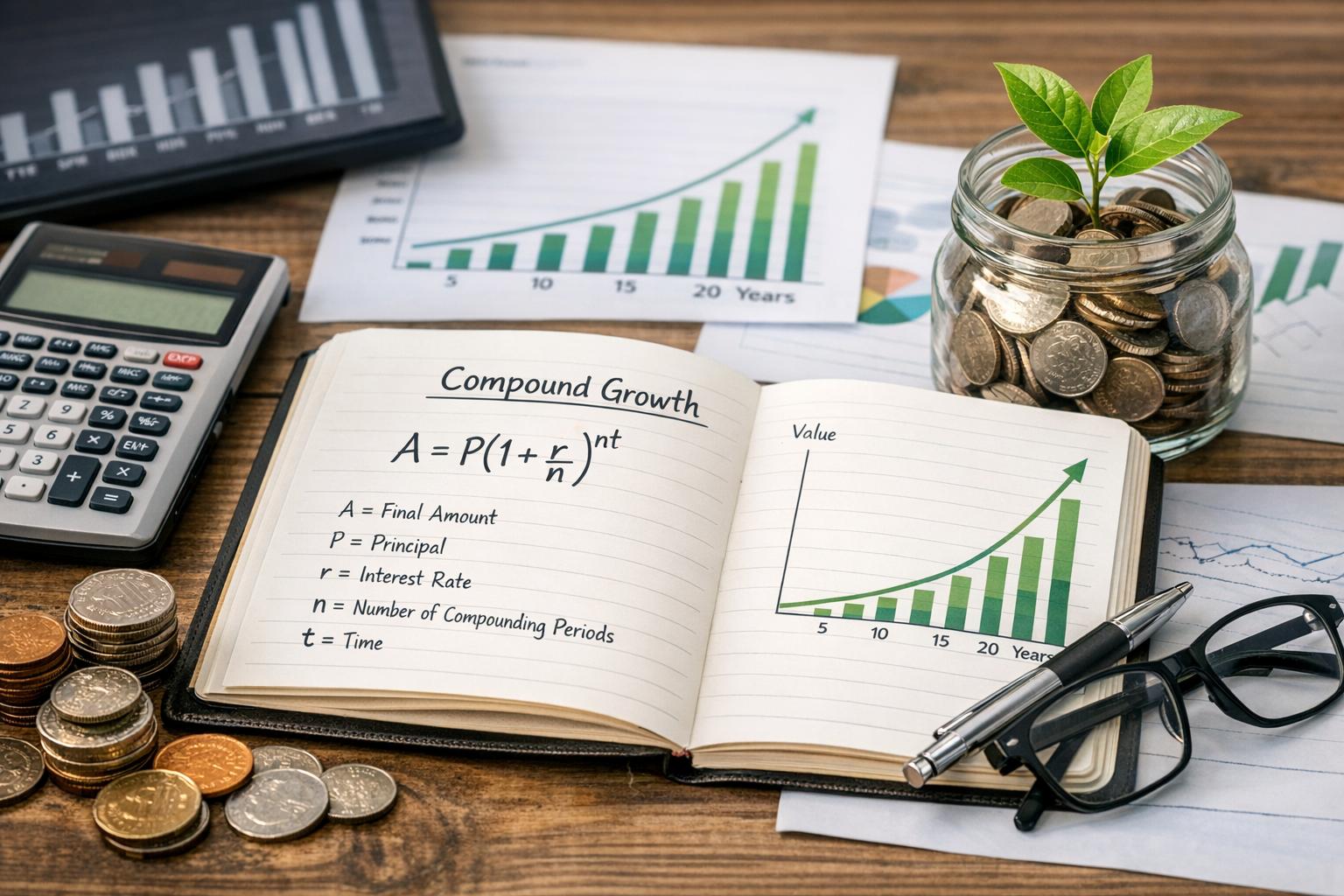
Compound growth is a mathematical process in which an amount earns growth on its original value and on gains accumulated during earlier periods. The same principle applies to savings interest, investment returns, inflation, business revenue, population change, and unpaid debt.
The defining feature is that each period’s gain becomes part of the base used for the next calculation. Early increases may appear modest, but later increases become larger when the rate remains positive. Simple growth behaves differently because it adds the same absolute amount during every period.
For traders and investors, compound mathematics provides a useful framework for measuring account growth, comparing returns, estimating future values, and assessing the effect of fees or losses. It does not predict market returns. Rather, it shows what happens when a stated sequence of percentage changes is applied to a changing balance.
Simple Growth and Compound Growth
Suppose an initial amount of $1,000 grows at 5% per year. Under simple growth, the annual increase is calculated only from the original $1,000. Five percent of $1,000 is $50, so the balance rises by $50 each year:
Year 1: $1,050
Year 2: $1,100
Year 3: $1,150
After three years, the balance is $1,150. The total increase is $150, equal to three annual increases of $50.
With annual compound growth, each increase is calculated from the current balance. The first year still adds $50. The second year adds 5% of $1,050, or $52.50. The third year adds 5% of $1,102.50, or $55.125:
Year 1: $1,050.00
Year 2: $1,102.50
Year 3: $1,157.63
The compounded balance is about $7.63 higher than the simple-growth balance after three years. That difference is small because the period is short. Over 20 or 30 years, the gap becomes much larger.
| Year | Simple growth | Compound growth |
|---|---|---|
| 0 | $1,000.00 | $1,000.00 |
| 5 | $1,250.00 | $1,276.28 |
| 10 | $1,500.00 | $1,628.89 |
| 20 | $2,000.00 | $2,653.30 |
| 30 | $2,500.00 | $4,321.94 |
The table assumes no deposits, withdrawals, taxes, or fees. It also assumes the 5% rate occurs every year. Real investment results rarely follow such a tidy pattern, but the comparison shows how repeated multiplication changes the result.
The Basic Compound Growth Formula
The standard compound growth formula is:
A = P(1 + r)t
In the formula, A is the ending amount, P is the principal or starting amount, r is the rate per period written as a decimal, and t is the number of periods.
If $2,000 grows at 4% per year for six years, the calculation is:
A = 2,000(1 + 0.04)6
The annual growth factor is 1.04. Raising it to the sixth power gives about 1.265319:
A ≈ 2,000 × 1.265319 = $2,530.64
The accumulated growth is about $530.64. A simple-interest calculation would produce only $480 because it would add $80 per year for six years.
The units of r and t must match. If r is a monthly rate, t must count months. If r is annual, t must count years. Mixing an annual rate with a monthly period count is a common spreadsheet error and can produce a wildly overstated projection.
The Growth Factor
The expression 1 + r is called the growth factor. A 4% gain has a factor of 1.04, while a 4% loss has a factor of 0.96. Multiplying a balance by the factor applies the percentage change once.
Growth factors also make multi-period calculations easier to read. If a trading account gains 3% in January, 2% in February, and 4% in March, the ending value of a $10,000 account is:
$10,000 × 1.03 × 1.02 × 1.04 = $10,926.24
The three-month return is 9.2624%, not exactly 9%. Each month’s return acts on the balance left by the prior month.
Why the Exponent Matters
The exponent represents repeated multiplication. At a 4% annual rate, the amount is multiplied by 1.04 once per year. Over six years, the factor is:
1.04 × 1.04 × 1.04 × 1.04 × 1.04 × 1.04
This repeated multiplication makes compound growth nonlinear. A graph of constant positive growth curves upward rather than following a straight line. The slope becomes steeper because the same percentage applies to a larger balance.
Time exerts much of its effect through the exponent. Doubling the holding period does not simply double the final gain. At 8% annually, $10,000 grows to about $14,693 after five years. After ten years it reaches about $21,589, which is more than twice the five-year gain.
The same structure describes a repeated decline. If an amount falls by 3% annually, the factor is 0.97:
A = P(0.97)t
A $10,000 balance subjected to a 3% annual decline for ten years would fall to about $7,374. The dollar decline becomes smaller each year because 3% is applied to a shrinking base. This process is often called exponential decay.
Writing Percentage Rates Correctly
A percentage must be converted to decimal form before entering it in a formula. A rate of 7% becomes 0.07, while 0.5% becomes 0.005. Entering 7 rather than 0.07 would imply a growth factor of 8, or a 700% gain per period. That is rarely the intended assumption.
For a positive return, add the decimal rate to 1. For a loss, subtract the decimal rate from 1. A 12% gain has a factor of 1.12, while a 12% loss has a factor of 0.88.
Opposite percentage changes do not cancel unless they are calculated in relation to the same starting base. A 20% rise followed by a 20% fall turns $100 into $96:
$100 × 1.20 × 0.80 = $96
The gain adds $20, but the later loss removes $24 because it applies to $120. The order of pure percentage returns does not change the final product when there are no cash flows. A 20% loss followed by a 20% gain also produces $96. Deposits and withdrawals can change that property because they alter the amount exposed to each return.
Losses and Required Recovery Returns
A loss requires a larger percentage gain to restore the original balance. If an account falls from $100 to $80, it must gain $20. Yet $20 is 25% of $80, so the required recovery return is 25%, not 20%.
The recovery rate after a loss L can be calculated as:
Recovery rate = 1/(1 − L) − 1
| Loss | Balance remaining | Gain needed to recover |
|---|---|---|
| 10% | 90% | 11.11% |
| 20% | 80% | 25.00% |
| 30% | 70% | 42.86% |
| 50% | 50% | 100.00% |
| 75% | 25% | 300.00% |
This asymmetry matters in trading. Large drawdowns reduce the capital base available for later gains. Risk control does not guarantee a profit, but avoiding severe losses can materially affect long-term compound results.
Compounding Several Times Per Year
Interest may be compounded annually, semiannually, quarterly, monthly, or daily. If the nominal annual rate is r and compounding occurs n times each year, the formula becomes:
A = P(1 + r/n)nt
The expression r/n gives the periodic rate, while nt gives the number of compounding periods.
Suppose $5,000 earns a nominal annual rate of 6%, compounded monthly, for four years. The inputs are:
P = 5,000
r = 0.06
n = 12
t = 4
The calculation is:
A = 5,000(1 + 0.06/12)12 × 4
A = 5,000(1.005)48 ≈ $6,352.45
If the same nominal rate were compounded annually, the result would be:
A = 5,000(1.06)4 ≈ $6,312.38
Monthly compounding produces about $40.07 more over four years because interest enters the balance sooner. The difference between compounding schedules tends to rise with the principal, rate, and holding period.
Compounding frequency should not be confused with payment frequency. A lender may calculate interest daily but collect payments monthly. A broker may accrue margin interest each day and post it to an account on another schedule. The account agreement defines how the balance is calculated.
Nominal Rates and Effective Annual Rates
A nominal annual rate does not always equal the actual one-year percentage increase. If compounding occurs more than once per year, the effective annual rate, or EAR, includes interest earned on earlier interest.
The formula is:
EAR = (1 + r/n)n − 1
For a nominal annual rate of 6% compounded monthly:
EAR = (1 + 0.06/12)12 − 1
EAR ≈ 0.061678 = 6.1678%
An account with this arrangement grows by about 6.17% during one year if the rate remains unchanged and no cash enters or leaves the account.
EAR permits a fairer comparison between products that quote different compounding frequencies. A 6% nominal rate compounded monthly pays a little more than a 6% rate compounded annually. By contrast, an advertised annual percentage yield generally already reflects intra-year compounding. Labels vary by product and jurisdiction, so the calculation basis deserves a careful read. Fine print earns its keep here.
Continuous Compound Growth
If compounding occurs continuously, the formula is:
A = Pert
The letter e is a mathematical constant with an approximate value of 2.71828. Continuous compounding represents the mathematical limit as the number of compounding periods becomes infinitely large.
If $1,500 grows continuously at 5% annually for eight years:
A = 1,500e0.05 × 8
A = 1,500e0.4 ≈ $2,237.74
Continuous compounding gives a slightly higher result than daily compounding at the same nominal rate. At ordinary interest rates, the difference is often small. The formula remains useful in economic models, option pricing, and calculations involving continuously compounded returns.
Continuously Compounded Returns
A continuously compounded return, also called a logarithmic return, is calculated as:
g = ln(A/P)
If a price rises from $100 to $110, the simple return is 10%, while the logarithmic return is:
ln(110/100) ≈ 0.09531 = 9.531%
Logarithmic returns can be added across time. If a security has daily log returns of 1%, −0.5%, and 0.8%, the three values sum to 1.3%. Simple returns must instead be combined through multiplication of their growth factors.
This additive property makes log returns useful in statistical work. They should still be distinguished from ordinary percentage returns, especially in reports intended for clients. A reader may reasonably assume that “return” means a standard holding-period return unless the method says otherwise.
Compound Growth with Regular Contributions
Many investment accounts receive repeated deposits. If an equal contribution is made at the end of every period, the future value of an ordinary annuity is:
FV = C[(1 + i)n − 1]/i
Here, C is the contribution per period, i is the periodic return, and n is the number of contributions.
Suppose an investor deposits $200 at the end of each month into an account earning 6% per year, compounded monthly, for five years. The monthly rate is 0.005 and there are 60 deposits:
FV = 200[(1.005)60 − 1]/0.005
FV ≈ $13,954.01
The investor contributes $12,000, while about $1,954 comes from growth under the constant-rate assumption. Actual investment returns change from month to month, so a real account will not follow the formula exactly.
If contributions occur at the beginning of each period, the arrangement is an annuity due. Each payment earns one extra period of growth:
FV due = C[(1 + i)n − 1]/i × (1 + i)
Using the same figures, beginning-of-month deposits would grow to about $14,023.78. The timing difference adds roughly $69.77 over five years.
Combining a Starting Balance and Contributions
An investor may begin with a lump sum and then make recurring deposits. The future value is the sum of the compounded principal and the annuity value:
FV = P(1 + i)n + C[(1 + i)n − 1]/i
If the account begins with $5,000 and receives the $200 monthly deposits described above, its projected value after five years is:
FV = 5,000(1.005)60 + 200[(1.005)60 − 1]/0.005
FV ≈ $20,698.26
This projection assumes deposits arrive on schedule and the rate never changes. Fees, taxes, skipped deposits, and market losses would alter the result.
Solving for the Growth Rate
Sometimes the initial value, final value, and time period are known, while the annual compound rate is not. Starting from:
A = P(1 + r)t
Divide by P, take the tth root, and subtract 1:
r = (A/P)1/t − 1
This rate is commonly called the compound annual growth rate, or CAGR. If an account rises from $20,000 to $32,000 in eight years:
r = (32,000/20,000)1/8 − 1
r ≈ 0.06054 = 6.054%
CAGR describes the constant annual rate that would connect the starting and ending balances. It does not claim that the account earned 6.054% during each individual year. The actual path may have included gains, losses, or long flat periods.
Solving for Time
The formula can also determine how long an amount takes to reach a chosen value. Beginning with:
A = P(1 + r)t
Divide by P and apply natural logarithms:
t = ln(A/P) / ln(1 + r)
To find how long $1,000 takes to reach $2,000 at 5% annual growth:
t = ln(2,000/1,000) / ln(1.05)
t ≈ 14.21 years
If interest is credited only at the end of each year, the balance would first exceed $2,000 after the fifteenth crediting date. If values accrue continuously within each year, the interpretation depends on the account’s calculation rules.
The Rule of 72
The Rule of 72 provides a quick estimate of doubling time. Divide 72 by the annual rate written as a percentage:
Estimated doubling time ≈ 72 / annual rate
At 6% annual growth:
72 / 6 = 12 years
The exact annual-compounding calculation is:
ln(2) / ln(1.06) ≈ 11.90 years
The approximation works reasonably well for many ordinary rates around 5% to 10%. At 2%, it estimates 36 years, compared with an exact result of about 35.00 years. At 20%, it estimates 3.6 years, while the exact result is about 3.80 years.
The rule can also estimate the effect of inflation. At 4% annual inflation, a price level would roughly double in 18 years. It is a mental shortcut, not a replacement for an exact calculation in loan documents, investment projections, or financial reports.
Arithmetic and Geometric Average Returns
Investment returns are often summarized with an arithmetic average. This is found by adding periodic returns and dividing by the number of periods. Compound performance requires the geometric average instead.
Suppose an investment gains 20% in one year and loses 20% in the next. The arithmetic average is zero:
(20% − 20%)/2 = 0%
Yet $100 becomes $96:
$100 × 1.20 × 0.80 = $96
The annualized geometric return is:
(0.96)1/2 − 1 ≈ −2.02%
The geometric average reflects the rate that compounds to the actual ending value. The arithmetic average can still be useful for estimating a one-period expected return, but it does not describe realized multi-period growth.
Volatility Drag
Variation in returns can reduce compound performance even when the arithmetic average looks respectable. Consider two accounts that both have an average annual return of 5% across two years.
Account A earns 5% in each year:
1.05 × 1.05 = 1.1025
Its two-year gain is 10.25%.
Account B gains 25% and then loses 15%:
1.25 × 0.85 = 1.0625
Its two-year gain is only 6.25%, although the arithmetic average remains 5%. This difference is commonly described as volatility drag. Greater variation does not automatically mean a poor investment, but return variability affects compounded wealth.
Sequence of Returns and Cash Flows
Without deposits or withdrawals, changing the order of periodic returns does not change the ending value. Multiplication is commutative, so 1.10 × 0.90 produces the same result as 0.90 × 1.10.
The order matters once cash flows occur. A large loss soon after a major deposit affects more money than the same loss before that deposit. This issue can appear in retirement withdrawals, managed accounts, and trading accounts that receive irregular funding.
Assume an investor starts with $10,000 and adds another $10,000 after the first year. If the account gains 20% in year one and loses 20% in year two, the calculation is:
($10,000 × 1.20 + $10,000) × 0.80 = $17,600
Reverse the returns and the result changes:
($10,000 × 0.80 + $10,000) × 1.20 = $21,600
The return factors are the same, but the later deposit experiences a different return. This is why account performance reports often separate investment performance from the effect of investor cash flows.
Time-Weighted and Money-Weighted Returns
A time-weighted return measures the performance of the invested assets while reducing the influence of external deposits and withdrawals. The calculation divides the measurement period at each cash flow, finds the return for each subperiod, and links those returns geometrically.
If the subperiod returns are 4%, −2%, and 3%, the linked return is:
(1.04)(0.98)(1.03) − 1 ≈ 4.98%
A money-weighted return accounts for both the size and timing of cash flows. It is the discount rate that sets the present value of contributions and withdrawals equal. In investment reporting, this is closely related to the internal rate of return.
Time-weighted performance is often used to assess a manager because the manager may not control client deposits. Money-weighted performance reflects the investor’s personal experience more directly. Neither measure is universally better; they answer different questions.
Inflation and Real Compound Growth
Nominal growth describes the change in the number of dollars, pounds, euros, or other currency units. Real growth adjusts for inflation and therefore relates more closely to purchasing power.
If an investment gains 7% while consumer prices rise by 3%, the real rate is not exactly 4%. The exact relationship is:
1 + rreal = (1 + rnominal)/(1 + rinflation)
rreal = (1.07/1.03) − 1 ≈ 0.038835 = 3.8835%
Direct subtraction gives a useful estimate, but division gives the exact compounded rate. Over one year, the gap may look minor. Over a long period, repeated differences accumulate.
If $10,000 grows at 7% annually for 20 years, its nominal value becomes about $38,697. If inflation averages 3%, the equivalent value in starting-year purchasing power is:
$38,697/(1.03)20 ≈ $21,421
The account has grown in real terms, but far less than the nominal balance alone suggests.
Fees, Taxes, and Trading Costs
Fees reduce the rate that compounds for the investor. If a portfolio earns 7% before an annual fee of 1%, a rough projection may use 6%. The exact result depends on how and when the fee is charged.
A $100,000 balance growing for 25 years at 7% would reach about:
$100,000(1.07)25 ≈ $542,743
At a net rate of 6%, it would reach:
$100,000(1.06)25 ≈ $429,187
The one-percentage-point annual difference produces a gap of more than $113,000 under these assumptions. The fee itself is only part of the cost; the investor also gives up future growth on money used to pay earlier fees.
Broker commissions, bid-ask spreads, financing charges, fund expenses, and currency conversion costs can have a similar compounding effect. Frequent trading may make small per-transaction costs matter more. Taxes can also interrupt compounding when gains are realized and tax is paid from the account.
Compound Growth in Debt
Compound mathematics applies to borrowing as well as investing. If interest is added to unpaid debt, later interest may be calculated on the accumulated balance. High rates can make balances rise quickly when payments do not cover accrued interest.
For a fixed-rate amortizing loan, the regular payment is commonly calculated with:
PMT = P[i(1 + i)n]/[(1 + i)n − 1]
Here, P is the loan principal, i is the periodic rate, and n is the number of payments.
Consider a $20,000 loan at a nominal annual rate of 6%, repaid monthly over five years. The monthly rate is 0.005 and there are 60 payments:
PMT = 20,000[0.005(1.005)60]/[(1.005)60 − 1]
PMT ≈ $386.66
Early payments contain a larger interest portion because the outstanding principal is higher. As principal falls, less interest accrues and more of each payment reduces the balance.
Credit cards and margin loans may use daily periodic rates, variable rates, minimum-payment rules, or transaction-based fees. Their balances may not fit a basic fixed-rate loan formula. The governing statement or agreement provides the applicable method.
Variable Returns and Compound Performance
Market returns rarely remain constant. If each period has a different rate, multiply the separate growth factors:
A = P(1 + r1)(1 + r2)(1 + r3)…
An investment that gains 10% in year one, loses 5% in year two, and gains 8% in year three has a total factor of:
1.10 × 0.95 × 1.08 = 1.1286
The cumulative return is 12.86%. Adding the rates gives 13%, which is close but not exact. The annualized geometric return is:
(1.1286)1/3 − 1 ≈ 4.12%
By comparison, the arithmetic average is about 4.33%. Compound analysis uses the geometric figure when describing the constant annual rate that matches the ending balance.
Common Calculation Errors
Several mistakes recur in compound-growth projections. One is using a percentage as a whole number rather than a decimal. Another is combining an annual rate with monthly periods without converting the rate.
Rounding too early can also distort long calculations. A periodic rate should generally retain several decimal places until the final result. The displayed answer may then be rounded to cents or to an appropriate percentage precision.
Other errors include treating average returns as compound returns, ignoring deposit timing, and assuming that fees can be deducted only once at the end. A projection may also present a constant return without stating that the rate is hypothetical.
Spreadsheet users should check cell references, exponent placement, and payment timing. In many financial functions, a payment entered as a positive number may produce a negative future value because the software treats contributions as cash outflows. The arithmetic may be correct even when the sign looks odd.
Limits of Compound Growth Models
A basic compound formula assumes a known rate that remains constant across regular periods. Actual investments, company revenue, inflation, and asset prices rarely behave with that consistency. Returns may vary sharply, and losses can occur.
The formula may also omit taxes, transaction costs, account fees, spreads, financing expenses, withdrawals, and contribution changes. A projection based on gross returns can therefore overstate the amount an investor keeps.
Market liquidity and execution also matter in trading records. A quoted market price does not always equal the price available for a large order. Back-tested returns may ignore slippage, delayed fills, or assets that ceased trading. Compound arithmetic can process the reported rates correctly while the input assumptions remain weak.
Future-value projections are models, not promises. Their value depends on transparent assumptions about the starting balance, return method, time period, compounding schedule, and cash-flow timing. A clean formula cannot repair poor data. Mathematics is fussy like that.
Applying Compound Mathematics Carefully
Compound growth is repeated multiplication. Each period’s ending balance becomes the next period’s starting balance, so gains, losses, fees, and inflation accumulate through time.
The expression P(1 + r)t describes a constant periodic rate applied to one starting amount. Variations of the formula account for recurring contributions, multiple compounding periods, continuous growth, loan payments, real returns, and changing rates.
For investment analysis, the rate definition matters as much as the formula. Nominal and effective rates are not interchangeable. Arithmetic averages do not represent compound performance. Time-weighted and money-weighted returns answer different performance questions, and a loss requires a larger percentage gain to recover.
Used with clear assumptions, compound mathematics offers a practical method for evaluating savings, investments, trading accounts, inflation, fees, and debt. It shows how balances change under stated conditions. Whether those conditions are realistic remains a separate analytical judgment.